Why use data from outside sources?

The world is awash in data, and whatever else we teach in a data science curriculum, data must be at the center. Calls to modernize statistics and data science courses regularly point to using “real” data. The National Academies Report on Data Science for Undergraduates (see previous blog post at: https://teachdatascience.com/nasem/) reports Data Management & Curation as a core part of data acumen. Indeed, they recognize data provenance to be a key skill which is “important for all students in [a] data science program.”

Additionally, students are typically much more engaged in the technical content if they are curious about the research question(s) posed by the data at hand. That is, if the students choose a particular dataset, they are more likely to spend time with the data practicing their data science skills. It is my experience that students are most likely to want to work with large datasets which speak to their daily lives. Capturing data from a website and making it usable in R can be a daunting task, but it is aided by R packages designed to ingest outside data into (mostly tidy) dataframes.

R packages for ingesting data from outside sources

• googlesheets: connect to googlesheets anywhere
• fivethirtyeight: connect to 538’s database
• jsonlite: parsing JSON data
• xml: parsing XML files
• datapasta: copy and paste for odd data structures in the wild
• rvest: package for scraping data from HTML pages
• httr: connect to APIs

The R packages described above require different levels of computational savvy. One might start with googlesheets and fivethirtyeight as a straightforward way to import data. Then jsonlite and xml help for downloading and more sophisticated parsing of the data structure. Finally, rvest and httr allow the R user to download data which exist in alternative structures (HTML pages or APIs). Below we walk through a complete example using googlesheets to download data from GapMinder.

Example using googlesheets to download literacy data from GapMinder

The example below comes from a project on creating Dynamic Datasets which was published in Technological Innovations in Statistics Education (Hardin, 2018). We import literacy rates measured at the country level from GapMinder via googlesheets. Note that non-public sheets requires an additional step of authentication, see googlesheets for more information.

Three datasets are loaded. The datasets are the female literacy rate over time, the male literacy rate over time, and the overall literacy rate over time for dozens of countries going back to the mid-1970s. The R code is given in the Markdown file.

# the URL for the GapMinder dataset(s) of interest
litF_url <- "https://docs.google.com/spreadsheets/d/1hDinTIRHQIaZg1RUn6Z_6mo12PtKwEPFIz_mJVF6P5I/pub?gid=0"
litM_url <- "https://docs.google.com/spreadsheets/d/1YF1_ps4srYp8GLdH38v7hJQtDDjFJWz6_5bg-_zICaY/pub?gid=0"
litALL_url <- "https://docs.google.com/spreadsheets/d/12O0Bo85Dd-9bNq6p5KwXduPET1cRETP-mKy3ZK4q_xo/pub?gid=0"


#pulling in the URL & keeping track of how big it is
litFurl <- googlesheets::gs_url(litF_url, visibility="public")
litF_nrow <- litFurl$ws$row_extent[1]
litF_ncol <- litFurl$ws$col_extent[1]

litMurl <- googlesheets::gs_url(litM_url, visibility="public")
litM_nrow <- litMurl$ws$row_extent[1]
litM_ncol <- litMurl$ws$col_extent[1]

litALLurl <- googlesheets::gs_url(litALL_url, visibility="public")
litALL_nrow <- litALLurl$ws$row_extent[1]
litALL_ncol <- litALLurl$ws$col_extent[1]


#reading in the datasets
litF <- googlesheets::gs_read(litFurl, range=googlesheets::cell_limits(c(1,1), c(litF_nrow,litF_ncol)))
litM <- googlesheets::gs_read(litMurl, range=googlesheets::cell_limits(c(1,1), c(litM_nrow,litM_ncol)))
litALL <- googlesheets::gs_read(litALLurl, range=googlesheets::cell_limits(c(1,1), c(litALL_nrow,litALL_ncol)))

Looking at the data at this point is a good idea. One thing to notice is that there is a ton of missing data. That’s expected (especially if you are used to looking at GapMinder data), because we wouldn’t expect that every country has literacy data for each gender going back 40 years for every single year. Also, notice that the data aren’t in tidy format (rows as observational units and columns of variables). After we wrangle the data below it will (a) look different and (b) be in tidy form.

glimpse(litALL)
## Rows: 260
## Columns: 38
## $ `Adult (15+) literacy rate (%). Total` <chr> "Afghanistan", "Albania", "A...
## $ `1975`                                 <dbl> NA, NA, NA, NA, NA, NA, NA, ...
## $ `1976`                                 <dbl> NA, NA, NA, NA, NA, NA, NA, ...
## $ `1977`                                 <dbl> NA, NA, NA, NA, NA, NA, NA, ...
## $ `1978`                                 <dbl> NA, NA, NA, NA, NA, NA, NA, ...
## $ `1979`                                 <dbl> 18.15768, NA, NA, NA, NA, NA...
## $ `1980`                                 <dbl> NA, NA, NA, NA, NA, NA, NA, ...
## $ `1981`                                 <dbl> NA, NA, NA, NA, NA, NA, NA, ...
## $ `1982`                                 <dbl> NA, NA, NA, NA, NA, NA, NA, ...
## $ `1983`                                 <dbl> NA, NA, NA, NA, NA, NA, NA, ...
## $ `1984`                                 <dbl> NA, NA, NA, NA, NA, 95.4071,...
## $ `1985`                                 <dbl> NA, NA, NA, NA, NA, NA, NA, ...
## $ `1986`                                 <dbl> NA, NA, NA, NA, NA, NA, NA, ...
## $ `1987`                                 <dbl> NA, NA, 49.63088, NA, NA, NA...
## $ `1988`                                 <dbl> NA, NA, NA, NA, NA, NA, NA, ...
## $ `1989`                                 <dbl> NA, NA, NA, NA, NA, NA, NA, ...
## $ `1990`                                 <dbl> NA, NA, NA, NA, NA, NA, NA, ...
## $ `1991`                                 <dbl> NA, NA, NA, NA, NA, NA, NA, ...
## $ `1992`                                 <dbl> NA, NA, NA, NA, NA, NA, NA, ...
## $ `1993`                                 <dbl> NA, NA, NA, NA, NA, NA, NA, ...
## $ `1994`                                 <dbl> NA, NA, NA, NA, NA, NA, NA, ...
## $ `1995`                                 <dbl> NA, NA, NA, NA, NA, NA, NA, ...
## $ `1996`                                 <dbl> NA, NA, NA, NA, NA, NA, NA, ...
## $ `1997`                                 <dbl> NA, NA, NA, NA, NA, NA, NA, ...
## $ `1998`                                 <dbl> NA, NA, NA, NA, NA, NA, NA, ...
## $ `1999`                                 <dbl> NA, NA, NA, NA, NA, NA, NA, ...
## $ `2000`                                 <dbl> NA, NA, NA, NA, NA, NA, NA, ...
## $ `2001`                                 <dbl> NA, 98.71298, NA, NA, 67.405...
## $ `2002`                                 <dbl> NA, NA, 69.87350, NA, NA, NA...
## $ `2003`                                 <dbl> NA, NA, NA, NA, NA, NA, NA, ...
## $ `2004`                                 <dbl> NA, NA, NA, NA, NA, NA, NA, ...
## $ `2005`                                 <dbl> NA, NA, NA, NA, NA, NA, NA, ...
## $ `2006`                                 <dbl> NA, NA, 72.64868, NA, NA, NA...
## $ `2007`                                 <dbl> NA, NA, NA, NA, NA, NA, NA, ...
## $ `2008`                                 <dbl> NA, 95.93864, NA, NA, NA, NA...
## $ `2009`                                 <dbl> NA, NA, NA, NA, NA, NA, NA, ...
## $ `2010`                                 <dbl> NA, NA, NA, NA, NA, NA, NA, ...
## $ `2011`                                 <dbl> 39.00000, 96.84530, NA, NA, ...

Each of the original googlesheets comes as a spreadsheet with country as the row and year as the column. R imports the years as column names (which are difficult to deal with as numeric column headers), and we need to gather the data into a format such that “Year” is one of the variable names. At the end of the wrangling process, the variables will be: country, year, litRateF, litRateM, litRateALL, and continent.

litF <- litF %>% select(country=starts_with("Adult"), everything()) %>%
        gather(year, litRateF, -country) %>%
        mutate( year = readr::parse_number(year)) %>%
        filter(!is.na(litRateF)) 

litM <- litM %>% select(country=starts_with("Adult"), everything()) %>%
        gather(year, litRateM, -country) %>%
        mutate( year = readr::parse_number(year)) %>%
        filter(!is.na(litRateM)) 

litALL <- litALL %>% select(country=starts_with("Adult"), everything()) %>%
        gather(year, litRateALL, -country) %>%
        mutate( year = readr::parse_number(year)) %>%
        filter(!is.na(litRateALL))

literacy <- full_join(full_join(litF, litM, by=c("country", "year")), 
                     litALL, by=c("country", "year"))

Now the data frame is in tidy format (rows are observational units, columns are variables), and the dataframe literacy has all of the information needed.

glimpse(literacy)
## Rows: 575
## Columns: 5
## $ country    <chr> "Burkina Faso", "Central African Rep.", "Kuwait", "Turke...
## $ year       <dbl> 1975, 1975, 1975, 1975, 1975, 1975, 1976, 1976, 1976, 19...
## $ litRateF   <dbl> 3.182766, 8.399576, 48.015214, 45.098921, 38.124870, 94....
## $ litRateM   <dbl> 14.52849, 29.59292, 68.02863, 77.50394, 58.38611, 93.388...
## $ litRateALL <dbl> 8.685145, 18.236172, 59.564392, 61.627683, 53.514879, 93...

As mentioned before, we wouldn’t really expect every country to have literacy data for every year. However, it is straightforward to tally how many observations per country and per year exist in the dataset, if desired.

Modeling the GapMinder literacy data

An introductory analysis considers gender differences in literacy rates and uses a linear model on the difference between female and male literacy rates across time. In a statistics or data science class, you can show a graphical representation and discuss model assumptions including sampling and independence of residuals. The model indicates that the difference between male and female literacy rates is shrinking over time. However, we worry about the effects of other variables and encourage a more complete analysis. Indeed, there may be large biases in our model if important explanatory variables have been left out.

It is vital to note that the data collected here (and on all of GapMinder) is observational. Causal mechanisms cannot be implied regardless of strength of correlation, and we recommend a conversation with students about the dangers of possible confounding variables that might explain any suggested causal relationships.

ggplot(literacy, aes(x=litRateF, y=litRateM)) + 
    geom_point(alpha=.75, aes(color=year)) + geom_abline(slope=1, intercept=0)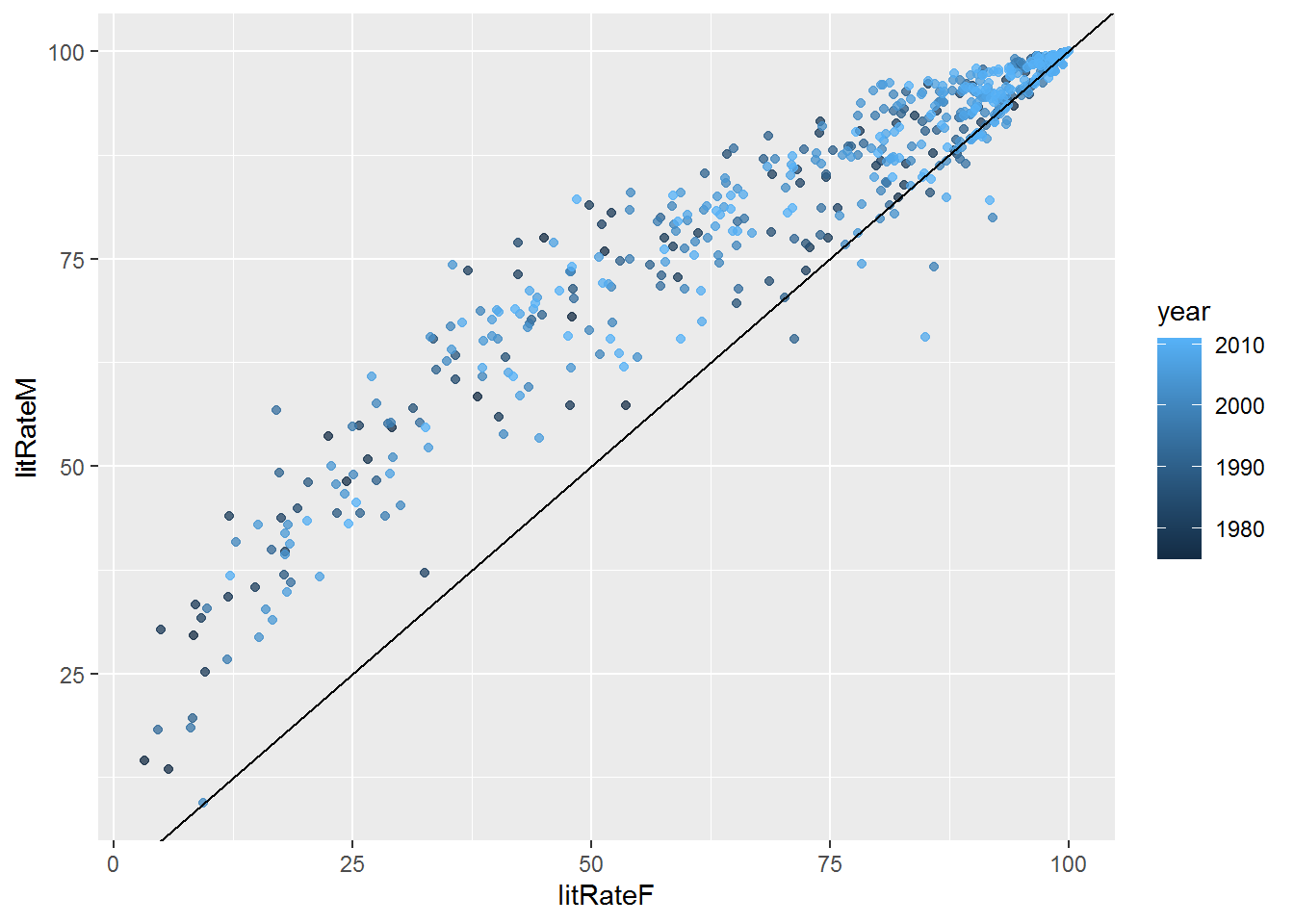

Figure 1: The plot shows that the higher the female literacy rate, the higher the male literacy rate. Additionally, across the board, the male literacy rate is higher than the female literacy rate (as referenced by the y=x line).

It might be interesting, however, to look at the relationship between literacy rates over time. To do that, we create a new variable which is the difference between male and female literacy rates.

literacy <- literacy %>% mutate(diffLit = litRateM - litRateF)
lm(diffLit~year, data=literacy) %>% tidy()
## # A tibble: 2 x 5
##   term        estimate std.error statistic     p.value
##   <chr>          <dbl>     <dbl>     <dbl>       <dbl>
## 1 (Intercept)  418.      80.1         5.22 0.000000256
## 2 year          -0.204    0.0401     -5.10 0.000000470