For the entire week, we’re going to be celebrating using Python for data science education. Stay tuned for topics on specific Python functionality, using Python inside RStudio, Python in the curriculum, and the larger Python community. But before we get to any of those topics, we’re going to start by introducing the go-to interface for Python programming, Jupyter Notebooks.
![]()
What is Project Jupyter?
Project Jupyter is a non-profit, open-source project, developed in 2014 out of the IPython Project and designed to support interactive data science and scientific computing across multiple programming languages. Because our blog introduced R Markdown (and implicitly R Notebooks) earlier, if you have not worked with Jupyter before then you might think of Jupyter Notebooks as being similar to R Markdown documents in many ways. There are differences, though; some of which will be described in this post.
More specifically, the Jupyter Notebook is an open-source web application that allows you to create and share documents which contain live code, equations, visualizations and narrative text. While the IPython Project focused on using Python, Jupyter initially evolved out of a broader sense of data science and scientific computer which involved the Julia, Python, and R languages. It has grown to accommodate over 40 programming languages (including SAS as well!), and there is now widespread support for viewing and working with Jupyter Notebook files on sites like GitHub and binder.
Working with Jupyter
Installing Jupyter is very easy with the few short steps outlined on the project’s install page. The base installation will provide access to the Jupyter Notebook interface for use with Python, to just create traditional text files, or to open a new terminal:
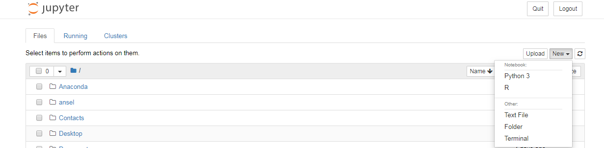
You will notice in the screenshot above that there is an option to start a new Notebook using R. We’ll get to this more in a bit. For now, observe the format of a Python kernel in a fresh Jupyter Notebook:
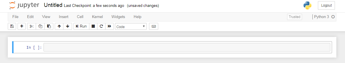
In Jupyter, the pieces are called “cells” as opposed to the “chunks” that exist in R Markdown, and a new Notebook is initialized with a single code cell. Cells can contain different types of things, most notably live code or narrative text. The “type” of the cell needs to be specified (note the small dropdown menu at the top center of the new Notebook screenshot that says “Code”) so that Jupyter knows how to treat (run or render) the contents of that cell. In its most raw, un-executed form a Notebook would look like the following:
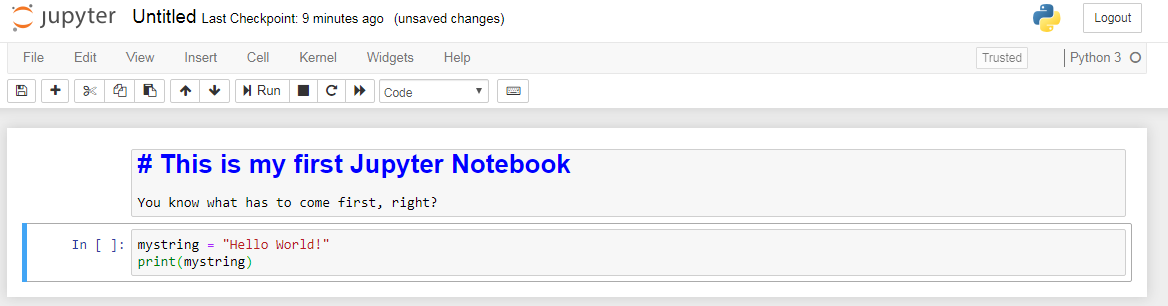
The Jupyter Notebook should be reminiscent of an R Markdown document. The first cell is text written in a markdown cell which supports plain text, markdown syntax, and even LaTeX syntax. The second cell is a code cell with a canonical first bit of code. Neither cell has been run at this point. There are dropdown menus and buttons at the top to run cells individually or many in sequence, but you can always execute the selected cell by hitting Ctrl + Enter. The first notable difference between Jupyter Notebooks and R Markdown documents is the ability to render markdown cells on-the-fly as opposed to needing to “Preview” or knit the whole document. Observe the result of “running” the first cell, but not the second:
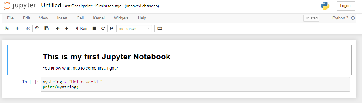
The heading and text are now appearing as if part of a “finished” HTML document, and we no longer see the raw cell structure. After running the second cell as well:
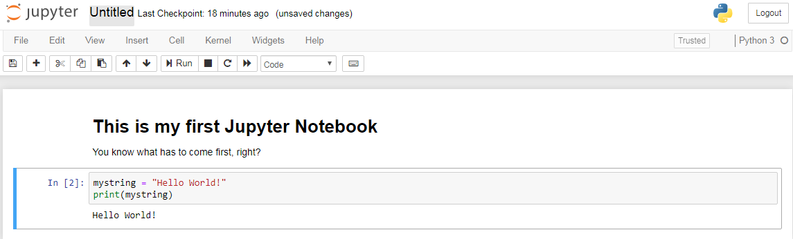
Similar to R Markdown (Notebook) files, the code cells produce output inline in the compiled document. The arrow buttons at the top of Jupyter Notebooks, however, allow for the user to rearrange cells at will without cumbersome copy-and-pasting.
Needless to say, Jupyter Notebooks provide an attractive and flexible alternative to RStudio to undertake interactive and reproducible data science work. They are an instinctive choice for many different projects when working in Python and many other languages including R, as you saw above. The choice between Jupyter and other tools such as R Markdown often depend on project specific details so make sure to check them all out so that you can choose what’s right for you.
Installing additional kernels (language support) for Jupyter is also relatively painless. The kernel for R can be found here on GitHub, and there are very nice instructions for getting R running in Jupyter in 3 easy steps.
Similar to R Markdown, Jupyter Notebooks are a great way to:
- deliver content to students,
- provide activities and assignment templates to students,
- allow students to undertake and submit their data science work.
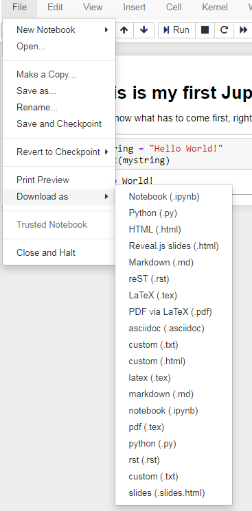
As a note on this last point, Jupyter Notebooks (or the output of them) can be downloaded in a number of different formats:
What is JupyterHub?
Put simply, JupyterHub “is a multi-user version of the notebook designed for companies, classrooms and research labs.” (JupyterHub homepage) JupyterHub runs in the cloud or on your own hardware, and makes it possible to serve a pre-configured data science environment to any user in your organization. It is customizable and scalable!
Despite how pain-free it is to set-up Jupyter on one’s personal machine is, JupyterHub streamlines the environment of your data science classroom. Instructors can maintain access to their students’ materials while students only have, say, write access to their own directories and read access to the instructor’s directory of materials. To this end, JupyterHub can be configured with authentication. (Setting up a JupyterHub is akin to serving RStudio in the cloud, as disucssed in our blog on RStudio in the cloud.)
The icing on the cake is the fact that JupyterHub is not limited to the Jupyter Notebook interface. It can be used to serve a variety of environments including RStudio!
As with the rest of the Jupyter Project, the JupyterHub technology is open-source and available on GitHub here.
Learn more
Project Jupyter Home: https://jupyter.org/index.html
JupyterHub Home: https://jupyter.org/hub
Data science with Julia: https://www.crcpress.com/Data-Science-with-Julia/McNicholas-Tait/p/book/9781138499980
Modularity and extensibility of Jupyter: https://blog.jupyter.org/99-ways-to-extend-the-jupyter-ecosystem-11e5dab7c54
The Jupyterhub Journey: Starting Small and Scaling Up A great video and blog about the JupyterHub story and use in UC Berkeley’s Division of Data Science and Information.
About this blog
Each day during the summer of 2019 we intend to add a new entry to this blog on a given topic of interest to educators teaching data science and statistics courses. Each entry is intended to provide a short overview of why it is interesting and how it can be applied to teaching. We anticipate that these introductory pieces can be digested daily in 20 or 30 minute chunks that will leave you in a position to decide whether to explore more or integrate the material into your own classes. By following along for the summer, we hope that you will develop a clearer sense for the fast moving landscape of data science. Sign up for emails at https://groups.google.com/forum/#!forum/teach-data-science (you must be logged into Google to sign up).
We always welcome comments on entries and suggestions for new ones.